How to Compare 2 Lists in Spreadsheets

How do I use spreadsheets to compare 2 lists and apply this knowledge to a practical framework? Let’s discover this while tackling the Gold Star Problem!

Compare 2 lists

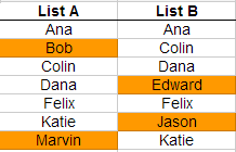
How can I use spreadsheets to indicate which names are not found in both lists? Seen to the left, the unique names (not common to both lists) are highlighted in orange. Is there a way to up the spreadsheet to create an efficient and automatic comparison between 2 lists? You bet!

Let’s discover this using an example: a Gold Star Problem.

Gold Star Problem

You are a club officer, and each club member can choose to participate in 3 volunteer activities. If the member participates in all 3, he or she receives a gold star. Given I have the attendance lists of each activity and the full membership list, who should receive a gold star?

If I have 10 club members, it is straight-forward to determine who receives gold stars. I simply look at the 3 sign-up lists and see whether each person’s name was present in all three lists. However, if I have 102 members, the process becomes far more time-consuming and laborious! Let’s figure out a way for the spreadsheet to compare 2 lists. Once we unlock this key, we can apply the formula across all 102 members.

View our 5-minute video tutorial below:

To compare 2 lists, we combine the ISNA and MATCH functions. The ISNA function returns a “TRUE” when it references an error or #N/A. So, =ISNA(#N/A) returns “TRUE.” Referencing anything else aside from #N/A will return a “FALSE.”

Now we can use the MATCH function as the reference, such as =ISNA(MATCH(A1, B:B, 0)).  The match function can determine whether the entity (or club member’s name) in cell A1 can also be found in column B. If the name is found in Column B, then the MATCH returns the row on which the name is found (let’s say it is 4), so ISNA(4) gives an output of FALSE. Conversely, if there is no match (i.e. the name in Cell A1 is not in column B), then the MATCH output is #N/A, so ISNA(#N/A) generates an output of TRUE.

In short, if the name is found in a volunteer activity list, then the ISNA/MATCH formula returns a FALSE. If the name is missing from the list, the formula returns a TRUE. We can apply this formula for each name across all 3 volunteer activity lists.

[googleapps domain=”docs” dir=”spreadsheet/pub” query=”key=0ArU-OSCYb_YpdHFscVZONGRsN3BIYVFpazFSenJqWVE&output=html&widget=true” width=”640″ height=”300″ /]

Once this step is completed, we have 3 columns that whether each person participated in each of the 3 volunteer activities. With this information, we can set up a formula (which I’ll let you figure out), to indicate whether the person receives a gold star (Hint: one way to solve this problem would be to use the IF and AND functions).

And there you have it! Once you master this, you can expand your spreadsheet by including formulas that determine who should receive a silver star (club member participates in 2 of the 3 activities), a bronze star (1 out of 3 activity), and a red warning (0 activity participation). At this point, you have built out a framework that automatically calculates what star status each club member receives.

Resources:

• Spreadsheet: How to Compare 2 Lists