Build a T-Ball or Softball lineup and positions generator

This season marks my youth softball coaching debut, an opportunity to impart my likely outdated baseball knowledge on a group of 5 and 6 year old girls. Beyond trying to stay positive and excited for an hour plus, the main challenge of coaching is organizing all the various tasks that come up.

One such task is setting a weekly lineup, which requires setting a batter order and assigning fielding positions by inning.

Some of the key rules that we’ll want to implement in the lineup:

  1. Randomize the batting order each week.
  2. Rotate the players on defense so that players don’t spend two innings in a row in the outfield, and the choice spots (pitcher, 1B) get fairly distributed.

Spreadsheet Logic

First we enter in all the names of the girls on the team, and for each week, we’ll assign a random number 1-10 which will be their spot in the order:

Then we can put them in order using Index(match):

Then we want to set up a rotation for the field – we use two columns, with the right column showing what position they will play after playing the left column. Players will rotate from LF to 3B to LCF to SS to RCF to 2B and so on:

We’ll then set the positions for the first inning, then for each subsequent inning, we’ll lookup the next position from the table above with vlookup:

And that’s the spreadsheet, you can check it out here: Softball Lineup Generator

To save a copy, go to File –> Make a copy

Dave and Busters breakeven tickets per chip under different chip cost and ticket value scenarios

Today we’ll continue with the theme from our last post on a Google Sheet Dave and Busters profitability tracker. One frequent question that arises in the Dave and Busters Reddit forum is: How many tickets does one need to be winning to be “profitable”?

The answer is usually some combination of “it depends”; it is based on chip cost and ticket value (and perhaps some mentions of finger traps, etc.).

To solve this problem, first we enter a formula for the breakeven tickets given a value/ticket and cost/chip. With some simple algebra, we find that:

breakeven ticket/chip = (cost per chip) / (value per ticket)

Here’s that depicted in spreadsheet form:

Next, we’ll make a data table which inputs various different costs per chip (based on the different price points of the tickets that are offered), and various different values per ticket. The output is this nice table below:

We can confirm we’re only an “advantage player” when it comes to redeeming for burgers and churros for ourselves at 10 tickets per chip breakeven.

Download the Excel spreadsheet here: Dave and Busters ticket breakeven calculator

You can also enter your own values in the Cost per chip (cells B26: B35) and Value per ticket (cells C25: J25).

Build a Dave and Busters tracker for chips spent, tickets earned and “profit”

This simple Google spreadsheet will help you keep track of your Dave & Busters visits and whether they were “profitable”.

Growing up, the local Tilt arcade was one of my favorite places to spent a weekend afternoon. As an adult, I remember being intrigued by an article on advantage players at Dave and Busters – people could win enough tickets to carve out some nice side income.

How many tickets do you need to win per credit played in order to be an advantage player? Today’s spreadsheet will solve that problem!

First, calculate what tickets are worth

We can figure out what tickets are worth by taking the value of a prize and dividing by the number of tickets. A YouTube tour of the Dave and Busters Ontario location from Arcade & Travel Adventures shows the prize center, which has an Oculus Quest 2 for 130k tickets, Airpods pro for 75k tickets.  Amazon has the Oculus Quest 2 for $400 and Airpods pro for $180.  The Oculus implies each ticket is worth 0.308 cents and the Airpods imply each ticket is worth .024 cents.

Next, calculate the cost of chips

The best deal appears to be paying $100 to get 750 chips.  This would result in a cost of about 13.3 cents per chip.

Finally, create the tracker

Our tracker will just be a simple ledger – the user will enter the date, the number of chips spent, and the number of tickets won. The spreadsheet will then calculate the value of the chips spent, the value of the tickets won, and the theoretical profit from the session. Over time by keeping track of all the sessions played, you can find out if you are profitable. Here’s how it looks, including one of my sessions at D&B where I “made” negative $7.88. Oh well, we’ll stick to the spreadsheets.

Check out the spreadsheet here: Dave and Busters Google spreadsheet tracker

Note: You can click File –> Save a Copy to save a copy for yourself to use.

Note 2: It looks like it takes about 43-44 tickets per chip in order to be “profitable” with the Value/ticket around 0.3 cents and Cost per chip around $0.13.

Run a tennis ladder with this Google Spreadsheet

In today’s post we’ll walk through how to build a weekly tennis ladder for a group of players. We’ll do it in Google Sheets, because we want players to be able to input the scores from their matches every time they play.

Each week we want players to enter in their scores, then move players up or down depending on if they won or lost, and then assign the players a new match for the next week.

Spreadsheet Inputs

We want a signup tab for players to enter in their name, contact information, and tennis skill level (We’ll use the NTRP rating system).

We’ll want to have a place each week for players to enter in who won and their match score (We’ll get to this later as we build the spreadsheet).

Here’s what we have so far:

Spreadsheet Outputs

First we sort the list by NTRP Rating and then add a new tab to paste the names in. For the first week’s match, we have #1 play #2, #3 play #4 and so on. We use the (semi) elegant formula isodd() to assign the matches with one formula pasted throughout. We use the next column to allow the players to check off who won, and then enter the score:


Then we add a column for week 2’s new rankings. Whoever wins moves up a rung, and whoever loses moves down. We use slightly different formulas for every other square to adjust the ladder for week 2. It’s easiest to just check out the spreadsheet yourself:

Our logic will be such that if you’re at the top and win, you get a bye and if you’re at the bottom and lose you get a bye so that the counting works out. We have to do slightly different logic and formatting every other week due to the top player in the ladder alternating between a bye and having a match.

After a little elbow grease and some formatting, here’s how our spreadsheet looks:

You can download the spreadsheet here: Google Sheets Tennis Ladder Spreadsheet

Remember: to use it you have to go to File –> Save a Copy. Then save a copy in your own Google Drive. Set the read/write permissions so anyone in your ladder or anyone with the link can read or edit. Hopefully, you don’t invite any sore losers who delete the whole spreadsheet!

What’s the expected value of your Mega Millions Ticket?

This spreadsheet follows the same logic as our previous post, What’s the expected value of your Powerball ticket?

First, we go to the Mega Millions website to look up the odds and the prize payouts for each combination of winning numbers:

We can use the same logic from our previous spreadsheet, and paste in the new odds, and convert them to probabilities (1 / (odds + 1)):

Looks like today’s jackpot of $122 million has only $0.65 of expected value per $2 ticket.

Check out the Excel spreadsheet here: Mega Millions Excel

We also put it on Google Spreadsheet here: Mega Millions Google Sheet

(Reminder, you can go to File –> Save a copy to download it to your Google Drive)

Set up fair teams using power scores from the last game

While the pandemic has been bad for physical fitness and social skills, it has been relatively good for various other endeavors – for me, guitar playing, tennis, chess, and Counterstrike:Global Offensive.

One of the problems that comes up in Counterstrike is how to set evenly matched teams when playing with a group of friends. We wouldn’t want to have captains and pick as people would feel bad to get picked last. We’d prefer to instead build a spreadsheet that uses the score from the previous game to set teams for the next game.

Spreadsheet Inputs

Previous game’s individual scores:

We’ve transcribed it into our spreadsheet as follows:

Next we’ll use some logic to sort the names by their scores:

Finally, we’ll assign each person to a team in order based on the power scores and the running tally of the total power score of the team. The spreadsheet checks to see which team has a current lower running total and adds the next player to that team until it fills up.

Check out the Google Sheets version here: Set Team Power Scores – Google Sheets

You can go to File –> Save a Copy to save it to your Google Drive to work with it on your own.

How to chart a tennis match with an Excel Spreadsheet

The return of live sports has been a welcome development during the COVID lockdown. We’ve enjoyed watching the US Open and seeing the new batch of young players that are going deep into the tournament.

Today’s post is for those parents who are dreaming of developing their kids into the next Roger Federer, Rafael Nadal, or more realistically (insert name of solid high school player who is able to get recruited into a highly ranked college).

The inspiration for this post comes from http://thetennisparentsbible.com/, a very in-depth (and intimidating) book on junior tennis development. One of the sections of the book is on match charting, or effectively keeping stats for your child’s match. Some of the benefits that author Frank Giampaolo cite are systematically evaluating performance, identifying strengths and weaknesses, and looking busy so you don’t have to talk to somewhat neurotic tennis parents (okay, I added the last one).
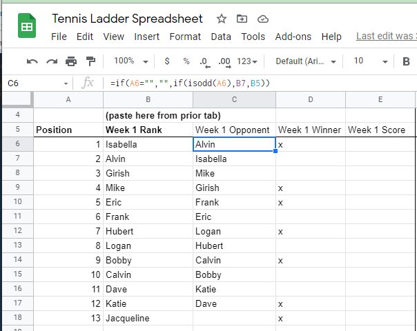
Spreadsheet Inputs

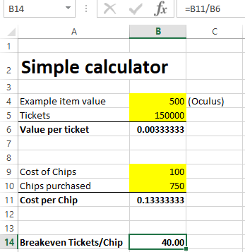
This spreadsheet is a bit tricky because of the amount of complexity that one could try for. In theory, every stroke could be a data point, including where on the court it was hit from, what spin it was hit with, and where on the court it was hit to. I’ll keep it relatively simple for now…

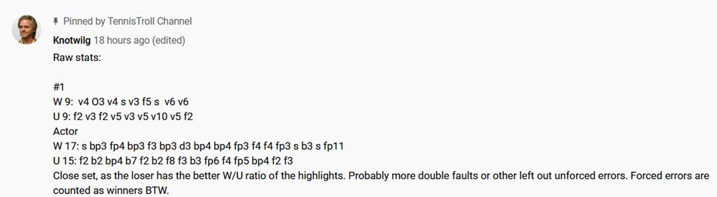
Basically we’ll keep track of who won the point, how many shots were in the rally, and how the point was won (winner or error, forehand or backhand, volley or groundstroke or serve). This system was inspired by someone named “Knotwilg” commenting on the TennisTroll Channel.

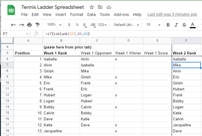
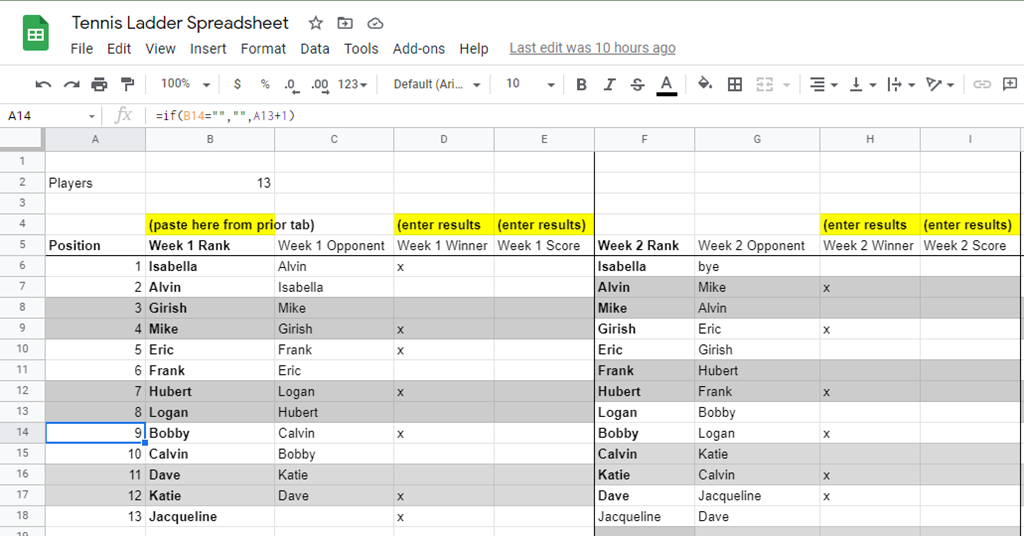
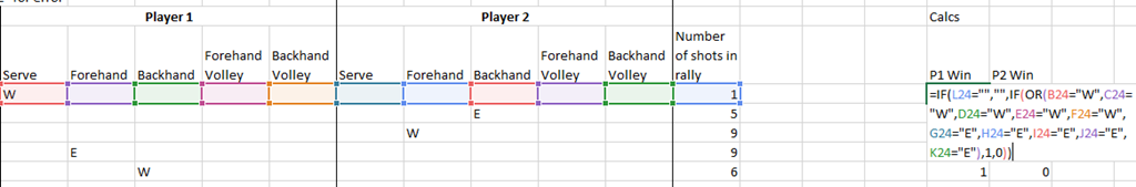
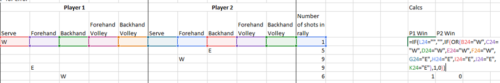
Here’s how our spreadsheet looks so far:

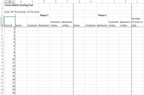
Here’s how I’d fill it out. If Player 1 hits an ace on the first point, I’d put a “W” into cell B6. Then if in the next point Player 2 dumps a forehand volley into the net, I’d put an “E” into cell J7. There will be lots of borderline situations (half volleys? forced error or winner? is a tweener a forehand or a backhand?), but out of simplicity we’ll keep it to just these five categories and winner or error, and let the user decide how to categorize the borderline cases.

Spreadsheet Outputs

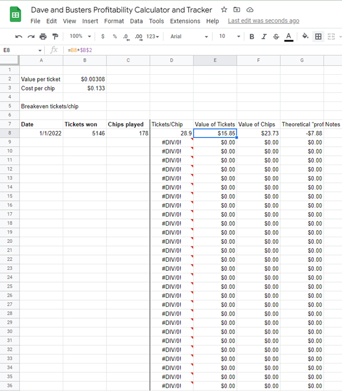
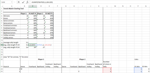
Now that we have some raw data of how all the points in a match were won or lost, we can create some summary statistics to give us some insights into how and why the match was won or lost.

I’ll insert some rows above the match chart to calculate some of these summary statistics. I’m sticking to the basics here – first we’ll count Player 1’s winners:

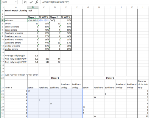
The other formulas follow similar logic and break it out by strokes.  We then add percentages to the winners versus errors.

Finally, we add some data on the rally length, including the overall average and the average rally length for when each player wins to give a sense of whether a player does better drawing out rallies or ending them faster. This includes adding an intermediate step of figuring out which player won the point:

And that’s pretty much it for this simple version of a tennis match tracker. In theory, you could customize for statistics you think are most important (like where on the court each player was to calculate things like net points won, etc). Also, one could build something that tracks matches over time. All great exercises for building your spreadsheet skills!

Download the spreadsheet here: Tennis Match Tracker

Build a Scrabble two and three letter word memorization training spreadsheet

While a big vocabulary is an important part of Scrabble success, an arguably more important Scrabble “skill” is memorizing all of the two-letter, and at a more advanced level, three-letter words. A well-played “QI” or “XI” or “QAT” can be the difference between winning and losing. This sheet is the adult version of last week’s Sight Words Quiz for kids.

In today’s post, we’ll build a quiz in which you can type in the first, second, or third letter, and the spreadsheet will return a random two or three letter word that matches the input.

Spreadsheet inputs

We’ll use a complete list of two and three letter words using this website. We’ll also add in a little logic in columns B-D that breaks out each word into its individual three letters, which we’ll need for later:

Note that we’ll start the data on line 15, since we’ll likely have our interface and some calculations in row 1-13. We’ll have separate tabs for our two-letter and three-letter quizzes. We went with Google Sheets so that in theory you could pull this sheet out on your phone during some downtime on the subway…whenever we’re able to ride those again…

Spreadsheet Calculations and Output

You can enter in any of the three letters in the words you want to pull, then put in some logic to assign a 1 to the words that match the user inputs and a 0 if they don’t match.

Here’s my attempt to explain what I did: Columns E,F,G check to see if each of your letters match the current word, and returns a 1 if it matches, 0 if it doesn’t. Column H checks to see if all three letters matched by seeing if E,F,G sum to 3. Column I assigns a unique number to each match, and then Column J cleans up Column I by setting all the non-matches to 0. Columns K and L look up all the matches in order.

It’s probably better understood if you download the spreadsheet and walk through the formulas.

Here’s what it looks like, and I pasted in what the key formulas look like in rows 11 and 12:

Note that this sheet provides a quiz, where one word is randomly drawn, but you can also just scroll through column L to see all the possible Scrabble words that match the search criteria.

Download the spreadsheet here (reminder, you can Make a copy of the spreadsheet and save it to your Google Drive by going to FIle –> Make a Copy:

Google Spreadsheet: Spreadsheet Solving Scrabble Quiz 

Here’s a Google Sheets tip: To generate a random number, you have to recalculate the Sheet. In Microsoft Excel, you just have to hit F9 to recalculate. In Google Sheets you can just hit Ctrl+R in any cell, which effectively copies the cell to itself, but also has the benefit of recalculating the sheet and generating a new random quiz word.

Build a Kids Sight Words quiz spreadsheet

Coronavirus lockdown week 11? – Let’s continue with what has now become a series of posts on educational kids activities spreadsheets. As a reminder, Part 1 was a Math Dice spreadsheet game and Part 2 was a Custom Math Worksheet Generator. Today’s spreadsheet will hop over to the English language part of elementary education and help you quiz your kids on their sight words.

Our goal is to take a list of sight words and randomly pull one word every time the sheet is refreshed so you can quiz your child. Sight words are frequently occurring words that kids should memorize rather than sound out.

Spreadsheet Inputs

  • The list of Dolch sight words. Edward William Dolch compiled this list of words, which were published in a journal in 1936.

  • The grade level. We’ll do a little trick here where we add a drop down menu by using the Data Validation function to select from the list of possible grade levels in the above screen, cells F4:F48.

Spreadsheet Output

Once you pick a grade level, the spreadsheet will use the Randbetween() function to generate a random number between 1 and the maximum number of words in that grade level. Then it uses a vlook function to return the word with which you can torture test your child.

Try it out yourself by downloading the spreadsheet here: Dolch Sight Words quiz spreadsheet. Remember to hit the F9 key to recalculate the worksheet and generate a new random sight word.

A simple scoreboard spreadsheet for lockdown Zoom games

Here’s a simple spreadsheet that serves as a handy scoreboard to keep track of who is winning your Zoom games. While there’s not much to it, feel free to save a copy to your Google Docs folder. We’ve been playing some Jackbox Party Pack, which keeps score for you, but I could see how there could be other situations (competitive Zoom rock paper scissors?) where you could have your own scoreboard.

Anyways, basically the only calculations involved are the Sum() and Rank() functions. I added in a little bit of formatting (freezing at Row 9 if the game goes many rounds, and shading every other row).

Stay Safe and enjoy!

Spreadsheet is attached here: Simple Scoreboard

(Remember to go to File –> Save a Copy to download a copy to your own Google Sheets Drive that you can Edit).

Build a “Math Dice” Mental Math Mobile Spreadsheet

I remember in 4th grade, a math teacher would write five numbers on the board and ask us to use addition, subtraction, multiplication and division to try arriving at a target number. Like many good things from my childhood, this game has been commercialized into “Math Dice”, where you pay $9.99 for $1.25 worth of dice.

With the help of the randbetween() function, we can create our own unbranded mental math game, fully customizable with the number of “dice” and how large the “dice” can get. We can make it in Google Sheets so you can have it in your pocket anytime the desire to unleash your mental math skills arises.

Spreadsheet Inputs

1) The number of dice/random numbers to use as raw material for calculations.

2) How big the dice/inputs are allowed to be.

3) How big the target number is allowed to be.

Here’s our spreadsheet so far:

Spreadsheet Calcs and Output

Basically, we’ll have a cell for each one of the “dice” that the user wants. The formula will first check to see if we have too many dice, then if not, we generate a random number between 1 and the “Maximum “Dice” Value” input. We then generate a random number for the target value at the bottom.

Here’s how the sheet looks. Also, 2 + (4 x 3) = 14, boom!

Check out the spreadsheet here: Math Dice Google Spreadsheet 

You can save a copy of it to your Google Docs Drive to edit it. Every time you alter the sheet, it will generate new random numbers.

Build a Super Bowl squares pool generator spreadsheet

Ah, the Super Bowl – the action, the excitement, the commercials? The only issue with the Super Bowl is for the 97% of Americans located outside of the two metropolitan areas surrounding the two teams playing, the outcome of the game doesn’t really matter as much. To fix that, we have gambling…specifically, the classic Super Bowl squares pool.

For those who are unaware, a Super Bowl squares pool is a 10×10 grid, where each person can purchase a space on the grid. The numbers 0-9 are randomly assigned for each axis with one of the two teams assigned to each axis. Prize payouts usually happen each quarter for the square that matches the ones digit of the actual in game score for each team.

This will be a simple spreadsheet for building a square pool on a Google Spreadsheet:

First, we highlight a 10 x 10 grid, and assign the teams to each axis:

Next, we can build our random 0-9 number generator, first we put the formula “=rand()” in each of the 10 spots, then we use the formula RANK() to rank the random numbers. We have to subtract 1 from the RANK() function because we want the numbers 0-9 while RANK() would produce numbers 1-10.

Do the same thing for the columns, set the stakes and the payout rules, let people pick what squares they want, and then have a “drawing.” The rand() function recalculates after every spreadsheet action, so you’ll want to have an official “next action is final” with everyone around, then immediately screenshot and print the whole table before it recalculates again. Or else people will be suspicious when you have all the 0’s and 7’s…

Here’s the link to the Google Spreadsheet: Super Bowl Squares Pool Generator. Remember, you can access it by going to File->Make a Copy