Need a way to track results and calculate power ratings for your tennis, ping pong, chess, or video and board game leagues?
As you might guess from much of the content posted over the past couple years, we at Spreadsheetsolving are huge fans of sports and games. There’s something about competition that sharpens the senses and motivates you to do your best. There’s also something satisfying about there being a clear winner and a loser when the game is over.
So what can you do when you’ve organized a group to play tennis, ping pong, magic, etc. and you want a system to track results and assign people ratings based on their match histories?
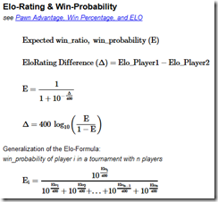
In Chess, a method called the Elo Rating System calculates relative skill levels: the difference between two players’ Elo Ratings tells you about the probability that one player will win, lose or draw. A beginner typically has an Elo Rating between 1000-1200 while Magnus Carlsen is around 2800. While the Elo System appears appealing, it seems very difficult to implement in a spreadsheet – we’re not really sure what to make of formulas like these:
Our ratings system will be much simpler and instead of fancy math, it’ll use the brute force method of the Solver function in Microsoft Excel.
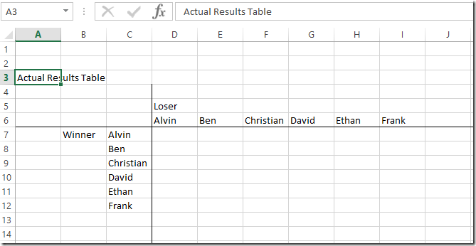
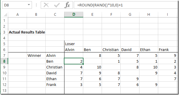
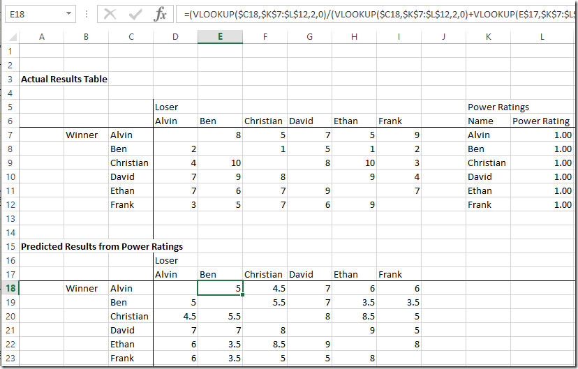
First, we create a table to track the actual win/loss results of the players in our ladder:
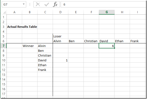
Now we can enter in the historical game data. Let’s say in the past 6 months, Alvin has won 6 times against David, and David has only one once against Alvin. We can enter this info like so:
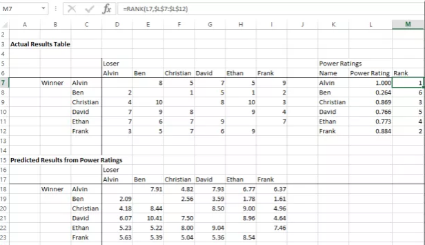
Now we’ll fill out the table with random data with the RAND() function and paste the values in to work with. Note the diagonals are left blank because the players wouldn’t play themselves. Just making sure we’re following along: David is 9 wins and 5 losses against Ben, Ethan is 7 wins and 10 losses versus Christian, Frank is 6 wins and 4 losses against David.
Now we want to determine a Power Rating for each player. Let’s use a simple rule that Player A’s probability of beating Player B can be determined by their power ratings by the simple formula of:
Probability of A Winning against B = Power Rating A / (Power Rating A + Power Rating B)
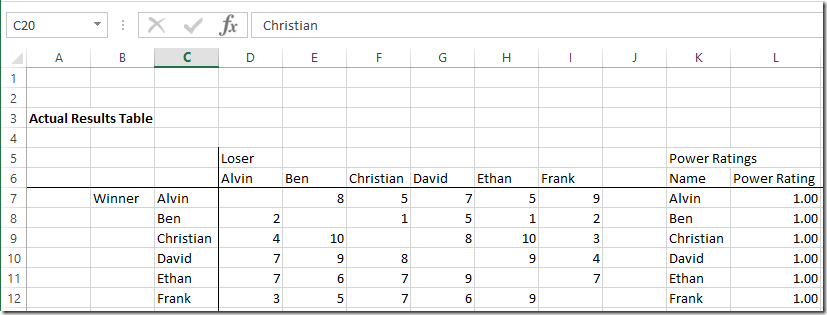
We add the starting Power Rating of 1.00 to Column K and L for each player,
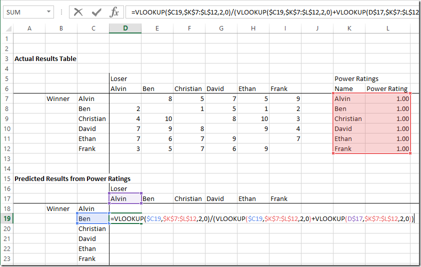
Then create a second table below with the predicted number of games won by each player against every other player based on the Power Rating win probability formula above multiplied by the total number of games played against each other player. This formula will get pretty involved with Vlookups() and relative cell references in order to paste the same formula across the whole table. Let’s break it down into two formulas for the predicted wins of Ben against Alvin:
The predicted percentage of games won by Ben vs Alvin. We lookup Ben’s and Alvin’s ratings in the table and do the appropriate calculation: =VLOOKUP($C19,$K$7:$L$12,2,0)/(VLOOKUP($C19,$K$7:$L$12,2,0)+VLOOKUP(D$17,$K$7:$L$12,2,0))
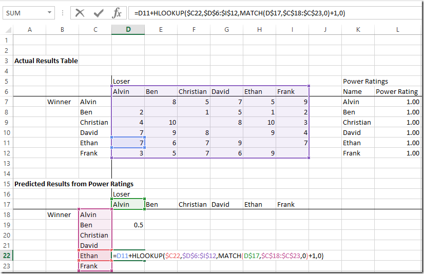
And then multiply that predicted percentage by the sum of the total number of actual games the two have played against each other. We use a Match function to tell the function to look down the correct number of spaces from the person we want: =D11+HLOOKUP($C22,$D$6:$I$12,MATCH(D$17,$C$18:$C$23,0)+1,0)
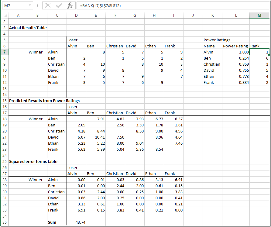
So we get the forecasted results from our initial power rankings of 1.00 for all the players. Notice we predict all of the players split the games played equally because everyone has the same power rankings for now:
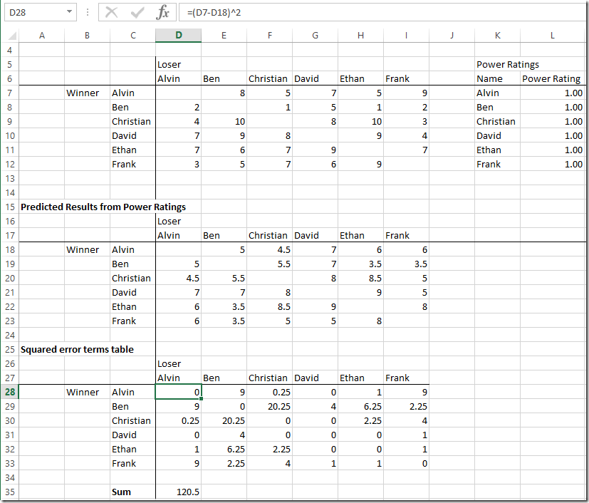
Then, we create a third table of “Error Terms” that takes the difference between the actual results and the predicted results from our power ratings. Given some errors are positive and some are negative and could cancel each other out, we square the errors to get all positive terms. Also, cell D35 takes the sum of all the squared errors:
Finally, we can employ the magic of the Solver function in Excel to calculate appropriate power rankings with the goal of minimizing the total error between the actual results and the predicted results from our power ratings. First, we have to open the Solver function. In our Excel, the Solver was inactive, so we activated it by going to File –> Options –> Add Ins
At the bottom, we clicked on the Manage: Excel Add-ins Go:
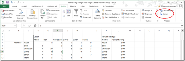
Then we checked the Solver Add-in and hit OK. Now it shows up as a function in the toolbar under the DATA tab:
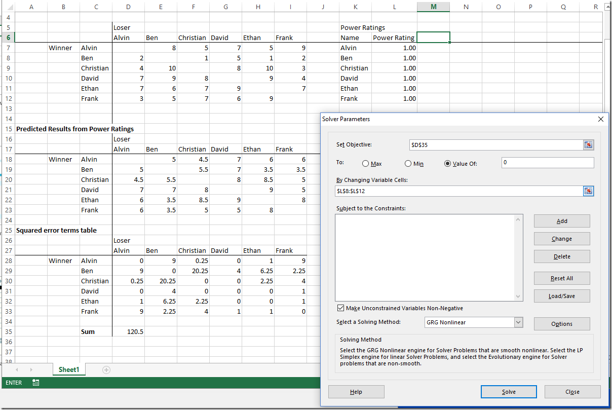
When you press Solver, it brings up the Parameters screen. We want to tell solver to minimize cell D35, which is the square of the errors, by changing the variable cells L8:L12, which are the Power Ratings. Note that we leave one person fixed at 1.00 so Solver has something to work off of:
Excel gives us an error, likely because the solution never gets to 0, but it does the best it can to produce a reasonable output. We can add the Rank() function to rank everyone according to their Power Ratings:
Good luck in your competitive endeavors. Hopefully this provides a tool to help give people skill ratings (and improve spreadsheet skills)!
Here’s the spreadsheet: Game and Sports Power Ratings

