Is the “height success rate” for seeds grown in organic soil significantly higher than that for those grown in the non-organic soil? Let’s use a statistical test to find out! But before we delve in, let’s review the amazing Central Limit Theorem (CLT). Why so remarkable, you may ask?
The beauty of this theorem is that regardless of the shape of the original population’s distribution, taking the averages leads to a normal distribution as the sample size increases. So, even if we have no idea what the population’s distribution looks like, we can still get information about it (as long as our sample size, n, is large enough!) CLT is essentially the reason we can actually perform the hypothesis test we’re about to explore below!
Performing a hypothesis test includes 4 steps:
- Define the hypothesis
- Calculate the test statistic
- Look up the p-value and compare it to a fixed significance level
- State conclusion
<< See our related posts on experimental design and inferential testing >>
Design and Conduct Experiments with Spreadsheets
Hypothesis Testing with Spreadsheets – Part I
Ready to begin our hypothesis test? Let’s go! Our 10-minute video on hypothesis testing can be found at the bottom of our post.
Define the Hypothesis
The first step is to define the hypothesis. This step is essential — we need to specify exactly what hypothesis or claim we want to test. The null hypothesis (Ho) is usually defined as an event that occurs by chance. In contrast, the alternate hypothesis (HA) means that the observations are the result of a real effect – not just pure chance. By the end, you will have figured out whether or not enough evidence exists to reject the null hypothesis in favor of the alternate hypothesis.
So, what will our null and alternate hypotheses be? Our null hypothesis states that there is no difference between the proportion of height success in the Organic group (Group A) and that in the Non-Organic group (Group B). In other words, both are equal. Our alternate hypothesis is that the proportion of height success in the Organic group is greater than that in the Non-Organic group.
Mathematically, these are shown as
- Ho: PA = PB
- HA: PA > PB
The alternate hypothesis can be one-sided ( PA > PB or PA < PB ) or two sided ( PA = PB ). In our case, we will test a one-sided alternate hypothesis.
Calculate the Test Statistic
We calculate a test statistic that will evaluate the evidence against the null hypothesis – this is why this step is also important!
How is a test statistic determined? While we will not go into the nitty-gritty here, we hope to provide a general understanding of its construction and encourage you to see additional resources at the bottom of our post.
To decide on an appropriate test statistic, we look to our null hypothesis and its assumptions for guidance. We know the following: based on our null hypothesis, we are testing whether our 2 samples (organic group vs. non-organic group) have equal proportions (height success rates). We previously verified in our last post that our sample size is sufficiently large for a z-test. Putting this together, the test statistic we will calculate is a 2 sample z-statistic of equal proportions.
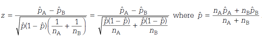
In general for a large sample, an approximately standard normal random variable (test statistic) is the difference in the sample “observed” proportion and the population “true” proportion, divided by the population standard error.
In our case, because we are comparing the difference of two sample proportions, the numerator of our test statistic is the observed difference of proportions minus the true difference of the population proportions. Now, we can actually simply this even more. How so? The null hypothesis that we defined above states that the population proportions are equal (i.e. the differences between them are zero). Therefore, for the numerator of our test statistic, we are left with the observed difference of proportions. You can see this reflected in the formula below.
Now how do we find the denominator or standard error? In general, the standard error for a single proportion test is the p (1 – p) divided by n. Because we have two samples and they are independent (as confirmed in our previous post), we can add the variances. Also, under the null hypothesis, proportions are the same, so we can pool the data to get the heights in both samples together. This is represented by the p-hat (as shown to the right of the formula). For those who are currently taking AP Statistics or a college-level introductory statistics course, the formula below may look familiar.
While it looks a bit involved, do not fret. Let’s use a spreadsheet and break it down into its component parts. The calculation is shown in the blue box below.
[googleapps domain=”docs” dir=”spreadsheet/pub” query=”key=0ArU-OSCYb_YpdFlONXY1WGNVVE1YU0VuSUM2YWYyMUE&output=html&widget=true” width=”640″ height=”384″ /]
Note: To view the spreadsheet, go to the Resources section below and click on the link. To edit it, first save the spreadsheet on your Google drive.
Look up the P-Value
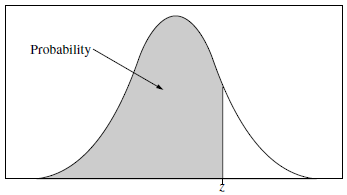
The p-value is a probability statement that answers the following question: If the null hypothesis were true, what is the likelihood of observing a test statistic at least as extreme as the one we observed?
So, that means that the larger the p-value, the stronger the evidence in favor of the Null Hypothesis. And vice versa: the smaller the p-value, the more the evidence points against the Null Hypothesis.
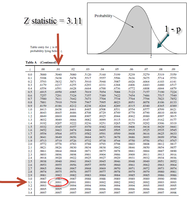
Using the z-table below, we look up the p-value (which is .9991), which represents the area under the curve along the left side of the distribution, as shown in the illustration. However, we are interested in the area in the far right-most tail, based on our alternative hypothesis (HA: PA > PB). So, the p-value can be calculated as 1 – .9991 or 0.0009, which is extremely small!
State our Conclusion
Finally, we can state our conclusion. In this case, we reject the null hypothesis, because the p-value of 0.0009 is very small and indeed smaller than any reasonable significance level, such as 0.05 or 0.01. Therefore, we can conclude that the proportion of plants who reach a height success of 15 mm or greater when given organic soil is significantly higher than that of plants who are assigned the non-organic soil!
Note: the data-set is not based on actual observations, so the conclusion is not accurate. Our goal was to demonstrate the process of hypothesis testing. If you are curious about this question, you now have the tools to design the experiment and test it using a hypothesis test!
Related Resources & Recommendations:
- Access and download this spreadsheet: Hypothesis Testing Spreadsheet
- Experimental Design: www.spreadsheetsolving.com/experiment-spreadsheet
- Hypothesis Testing I:www.spreadsheetsolving.com/hypothesis-testing1
- Video Tutorial: Design Experiments with Spreadsheets (7:46 min)
- Khan Academy: Hypothesis Testing with Two Samples