Printable Math Facts flash cards for single digit addition and subtraction with carrying

As kids start to add and subtract bigger and bigger numbers, they will have to learn how to “carry” a 10 when adding two numbers that sum higher than 10, and “borrow” a 10 when subtracting a bigger number from a smaller number.

Today’s spreadsheet is an example case of our Printable Flash Cards Spreadsheet, where we put in all the addition and subtraction math facts that students will need to know quickly in order to do longer addition and subtraction problems that may need carrying and borrowing.

Check out the spreadsheet here: Printable Flash Cards

To print – print double sided, and flip on the long edge. There are two tabs (“cards1” and “cards2”) with 72 total flash cards to print. Wish we had some good advice for how to get your kids to actually practice with these…

Understand and estimate your taxes with this spreadsheet

Tax day is coming up, and like many other families we plug a bunch of numbers into our tax software and pay/receive whatever it tells us to do. While this is effective, it doesn’t allow for much understanding of what is going on behind the scenes of how the numbers are calculated.

Also, if a family has two earners, this spreadsheet could help explain why there was a refund/underpayment by breaking out the federal and state tax rate each person paid, and compares that to what the tax rates were overall for the couple.

We repurposed the spreadsheet used for our post Will the Tax Cuts and Jobs Act make you pay more or less in taxes?, so look there for more details on how it was built. Note that this spreadsheet only works for a married couple filing in California (feel free to tweak it for your own needs. Also of course this is highly simplified with no investment income, etc).

Here’s an example, we filled in $100k income for person 1, $20k federal withholding, and $5k state withholding from their W2.  We also filled in their spouse’s $50k income and withholding, along with 12k in mortgage interest, $6k in property tax and $500 in charitable contributions, along with 2 kids”:

They would have owed roughly $18.7k in federal tax and $5,322 in state tax, for a 12.5% federal rate and 3.5% state rate.  We can see both spouses over-withheld by 7.5% and 3.5% roughly in this fictional example.

Check out the spreadsheet here: Tax Estimator

A “Put the numbers in order” Math Worksheet Generator spreadsheet

This spreadsheet builds upon our previous similar math worksheets: Find the pattern and fill in the blanks and Use the input dice to get the target number.

In this printable math worksheet generator, the user/teacher would enter in two inputs: how many numbers to order and how large the numbers can be. Then, the spreadsheet does the rest and generates 7 problems for the student to practice ordering a series of numbers.

Download the spreadsheet here: Put the Numbers in Order!

Our analysis of the $80k SALT deduction increase in the House BBB bill

We’ve had four years to mentally recover from building our analysis of the tax effects of the Tax Cuts and Jobs Act (TCJA) on a family in California. That post and the (extremely free and educational) downloadable spreadsheet highlight the power of spreadsheets and problem solving: we can figure out exactly what the tax change would be on a family in California.

Rather than guessing and hand-waving at the net effects of the bracket changes, AMT changes, and State and Local Tax (SALT) deduction changes, we showed that taxes would go up on California families earning over $700k.

So here we are again, with the House passing a version of the Build Back Better legislation, which includes an increase in the SALT deduction limit from $10k to $80k. Senator Sanders calls this a “tax break for the rich”.

We updated our spreadsheet with a third series of columns calculating federal taxes for our hypothetical California family (owns home worth 4x income, 3% mortgage, 1% property tax, 1.5% charity, etc. – you can change your assumptions as you wish) with the $80k SALT deduction. Usually on this website, we walk through step by step how the spreadsheet was built, but it is a little too involved here and easier for you to download the spreadsheet.

The first conclusion is yes, higher-income families benefit from the increase in the SALT cap. Generally, the benefit starts around $200-250k and maxes out around $1MM in income around $27k in tax savings:

But, let’s not forget that when TCJA was enacted and the SALT deduction was capped at $10k, these same higher income families in higher tax states faced a massive tax increase while taxes were cut everywhere else. For example, at $2.5MM income the tax increase was $92k, or about 3.7% of income:

Finally, if we look at the net effect of how taxes on higher income families in high tax states are doing after the House BBB SALT cap increase to $80k and TCJA together, there is still net a big tax increase on the rich, but slightly reversed by this legislation:

Download the spreadsheet here: Spreadsheet Solving BBB SALT Cap Analysis

A "Math Dice" inspired Printable Math Worksheet

Here’s another printable worksheet in our series of educational kids spreadsheets.  Today’s worksheet will revisit our “Math Dice” inspired spreadsheet game post that is now turned into a printable worksheet. We tend to like math activities in which kids are problem-solving and re-arranging numbers on the fly with many possible right answers, versus the standard computational “one right answer” spreadsheet.

The layout of this spreadsheet is similar to our original Pattern Recognition spreadsheet. Anyone can select up to 7 “dice” with the 8th number as the target. We’ll save you the gory details into how we used the rand() function and how we applied the formatting….and simply share the spreadsheet so you can start using it!

Try our Math Dice inspired printable worksheet.

A Custom Math Worksheet–arithmetic fill in the blanks

Today’s spreadsheet is a twist on our original Math Worksheet Generator Spreadsheet…..with a slightly more advanced variation!

Instead of (number) + (number) = fill in the answer, one of the addends or the answer itself will be randomly blank, and the student will have to fill in the missing value. 

We’ll spare you the gory details of how we adjusted our old spreadsheet to make this new spreadsheet (for each problem, we added in a random number 1-3, and then made the visible problem take either a blank or the actual number, and then added plenty of formatting).

Here’s the spreadsheet. Share your thoughts with us! 

The Bank for Kids – an educational bank ledger spreadsheet for parents

According to Scholastic, the recommended age to start giving kids an allowance is around 5-6 years. As parents of kids around that age, this makes sense: our kids are learning about coin values in school and starting to ask questions like “why can’t I buy a museum gift shop stuffed animal when you just spent four times that amount on groceries?”

With this newfound weekly cash flow, it’s a good time to introduce the concept of spending vs. saving, which is the cornerstone of many personal finance websites. When kids save, I suppose they could just keep the cash in a jar, but a more effective teaching tool would be to have them deposit it in the “Bank of Mom and Dad”, for not only safe-keeping, but also to earn an interest return on that saved money. The hope would be to illustrate the value of saving and for that savings to be “put to work” in generating even more money for them from interest.
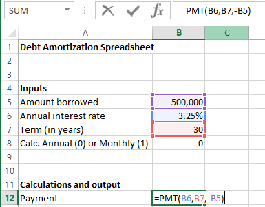
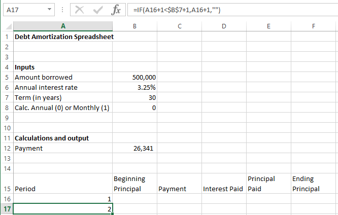
Spreadsheet Inputs

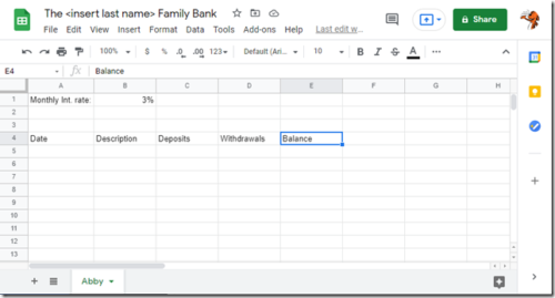
We’ll use Google Sheets for today’s spreadsheet with the thought that we’d like our kids to view the spreadsheet (but of course not edit…).

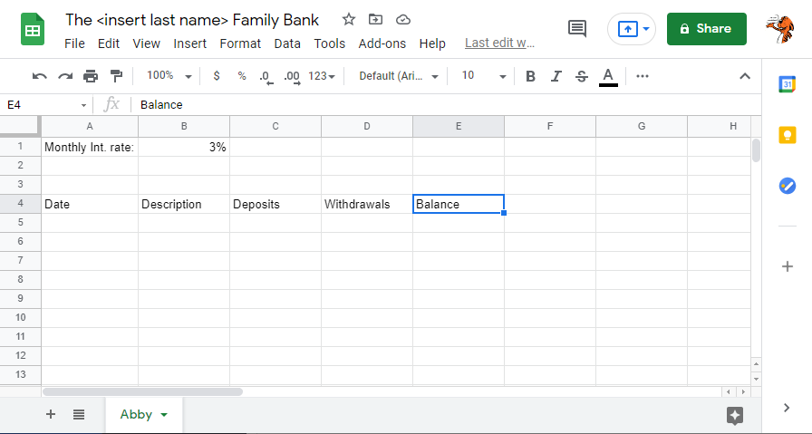
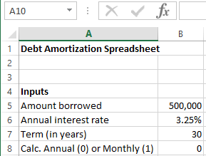
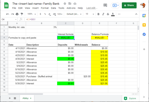
We’ll set the spreadsheet up like one of the old “passbook accounts” that I had as a kid (and from which my subconscious is likely drawing this post from):

Passbook - Wikipedia

We’ll also have an input for the monthly interest rate. This is an interesting decision as real monthly interest rates are perhaps only 0.04% and may not actually entice your child to save any money to earn no interest. I’ll put in 3% in our example. If little Abby finds a way to borrow a million dollars at 1% and put it in our bank, we might go bankrupt (although that’ll be promising for her Wall Street career…).

Here’s how our spreadsheet looks so far:

Spreadsheet Logic and output

There’s not really much to the logic: the Date, Description, Deposit, and Withdrawal items will typically be manual inputs depending on what is happening (allowance, withdrawal to buy stuffed animal, gift from Grandma, etc.).

The balance will just be a formula (last balance + deposits – withdrawals).

For interest payments, the formula will go in the deposits. One complication is whether to pay a full month’s interest on money that was deposited during the month by just using the last balance for the interest payment. In the name of simplicity, I think that’s fine. If little Abby figures out a way to arbitrage you by putting a lot of money in on the 30th of the month and then taking it out on the 1st…her financial education would be complete.

Check out the spreadsheet here, The Family Bank. Save a copy by going to File – > Make a Copy

Create and print physical flash cards with this Microsoft Excel template

Today’s spreadsheet will allow users to create 36 flash cards on one page with two-sided printing. We first tackled the idea of spreadsheet flash cards with this post on virtual flash cards, and today’s spreadsheet will tackle physical, printable cards.

We’ll have a separate sheet for our questions, which will feed into a sheet with our flash cards:

Then we’ll make our flash cards. First, we hit the print function, in order to show the dotted page lines. Then we sized the cards into a 9×4 grid, merging and centering cells, and adjusting the box widths to fill in the page lines. Finally, we linked the cards to the question and answer cells from the ‘questions’ tab. This was a little tricky as when you print two-sided the answers need to be flipped across the middle in order for them to match up with the questions:

That’s pretty much it – download the spreadsheet and try it out for yourself! Flash Card Spreadsheet in Excel

To print the flash cards, you’ll have to use the print option: Print on Both Sides –> flip pages on long edge.

We added some ideas for various flashcards:

  • Single digit numbers that sum to double digits
  • US States, State Capitals, Population
  • African/European States/Capitals

Run a tennis ladder with this Google Spreadsheet

In today’s post we’ll walk through how to build a weekly tennis ladder for a group of players. We’ll do it in Google Sheets, because we want players to be able to input the scores from their matches every time they play.

Each week we want players to enter in their scores, then move players up or down depending on if they won or lost, and then assign the players a new match for the next week.

Spreadsheet Inputs

We want a signup tab for players to enter in their name, contact information, and tennis skill level (We’ll use the NTRP rating system).

We’ll want to have a place each week for players to enter in who won and their match score (We’ll get to this later as we build the spreadsheet).

Here’s what we have so far:

Spreadsheet Outputs

First we sort the list by NTRP Rating and then add a new tab to paste the names in. For the first week’s match, we have #1 play #2, #3 play #4 and so on. We use the (semi) elegant formula isodd() to assign the matches with one formula pasted throughout. We use the next column to allow the players to check off who won, and then enter the score:


Then we add a column for week 2’s new rankings. Whoever wins moves up a rung, and whoever loses moves down. We use slightly different formulas for every other square to adjust the ladder for week 2. It’s easiest to just check out the spreadsheet yourself:

Our logic will be such that if you’re at the top and win, you get a bye and if you’re at the bottom and lose you get a bye so that the counting works out. We have to do slightly different logic and formatting every other week due to the top player in the ladder alternating between a bye and having a match.

After a little elbow grease and some formatting, here’s how our spreadsheet looks:

You can download the spreadsheet here: Google Sheets Tennis Ladder Spreadsheet

Remember: to use it you have to go to File –> Save a Copy. Then save a copy in your own Google Drive. Set the read/write permissions so anyone in your ladder or anyone with the link can read or edit. Hopefully, you don’t invite any sore losers who delete the whole spreadsheet!

What’s the expected value of your Mega Millions Ticket?

This spreadsheet follows the same logic as our previous post, What’s the expected value of your Powerball ticket?

First, we go to the Mega Millions website to look up the odds and the prize payouts for each combination of winning numbers:

We can use the same logic from our previous spreadsheet, and paste in the new odds, and convert them to probabilities (1 / (odds + 1)):

Looks like today’s jackpot of $122 million has only $0.65 of expected value per $2 ticket.

Check out the Excel spreadsheet here: Mega Millions Excel

We also put it on Google Spreadsheet here: Mega Millions Google Sheet

(Reminder, you can go to File –> Save a copy to download it to your Google Drive)

Build a debt amortization spreadsheet

The topic of debt can lead to some heated debate within the personal finance community. While some shun it, others see the value in borrowing for certain things, such as a house, education, a new tv (okay maybe not the tv). While this isn’t exactly a personal finance website, we can use spreadsheets to help visualize how much future money will be needed to repay the loan.

Today’s spreadsheet will walk through how to create a debt amortization spreadsheet. It will take a user’s inputs such as the amount borrowed, interest rate, term, and spit out an interest and payment table.

Spreadsheet Inputs

  • The amount borrowed, which is also known as the “principal.” This is the total loan amount.
  • The annual interest rate, which is about 3% for mortgages these days.
  • The term, which is the number of months or years over which you are borrowing.
  • Whether you want to calculate your payments monthly or annually.

Here’s what we have so far:

Spreadsheet Calculations and Output

The real magic of calculating debt payments is in the finance function PMT(). This function will take your principal, interest rate, and term, and calculate the level amortizing periodic payment. Here’s how we use it in our spreadsheet to calculate the annual payment for our example mortgage:

Next we make a schedule of each of the payment periods, where we keep a running tally of the beginning principal owed, the interest paid, the principal paid, and the ending principal owed.

Now we fill out the table. The first beginning principal comes from cell B5, the payment comes from cell B12, the interest paid is calculated by multiplying the beginning principal with the interest rate, the principal paid is the difference between the payment and interest paid, and the ending principal is the beginning principal minus the ending principal. The next period’s beginning principal is the previous period’s ending principal.

Was that clear?

That’s pretty much it. Feel free to walk through it yourself. I added in the logic to make it flexible for monthly or annual calculations.

Excel: Debt Amortization Spreadsheet

Google Sheets: Debt Amortization Spreadsheet  (you can go to File –> Save a Copy to copy it to your Google Drive to edit it)

Set up fair teams using power scores from the last game

While the pandemic has been bad for physical fitness and social skills, it has been relatively good for various other endeavors – for me, guitar playing, tennis, chess, and Counterstrike:Global Offensive.

One of the problems that comes up in Counterstrike is how to set evenly matched teams when playing with a group of friends. We wouldn’t want to have captains and pick as people would feel bad to get picked last. We’d prefer to instead build a spreadsheet that uses the score from the previous game to set teams for the next game.

Spreadsheet Inputs

Previous game’s individual scores:

We’ve transcribed it into our spreadsheet as follows:

Next we’ll use some logic to sort the names by their scores:

Finally, we’ll assign each person to a team in order based on the power scores and the running tally of the total power score of the team. The spreadsheet checks to see which team has a current lower running total and adds the next player to that team until it fills up.

Check out the Google Sheets version here: Set Team Power Scores – Google Sheets

You can go to File –> Save a Copy to save it to your Google Drive to work with it on your own.